Analysis workflow • mitodrift

This article walks through the standard post-inference analysis workflow: annotated tree → diagnostic PR curve → confidence trimming → clone assignment → visualization.

Core concepts for interpretation

Initial tree topology: a point-estimate starting tree constructed using neighbor joining (NJ) on continuous VAF matrices. This provides a fully-resolved (binary) initialization that empirically captures strong lineage signal before posterior sampling.
Posterior clade support: per-node support values in tree$node.label (0–1) estimated from MCMC topology sampling.
Confidence-based topology refinement: collapse internal edges below a support cutoff τ to obtain a refined lineage tree.

Setup

library(mitodrift)
library(data.table)
library(ggplot2)
library(dplyr)
library(patchwork)

We use a small in vitro LARRY barcode sample (200 cells, 186 variants) bundled with the package.

Run the same inference command used in the README:

Rscript inst/bin/run_mitodrift_em.R \
  --mut_dat inst/extdata/pL1000_mut_dat.csv \
  --outdir mitodrift_demo \
  --tree_mcmc_iter 5000 \
  --tree_mcmc_chains 4 \
  --tree_mcmc_burnin 1000

This writes mitodrift_demo/mitodrift_object.rds and mitodrift_demo/tree_annotated.newick. The workflow below uses the same mutation table and an annotated tree generated with those settings.

mut_dat <- read.csv(
  system.file("extdata", "pL1000_mut_dat.csv", package = "mitodrift")
)
data(pL1000_tree_annot)
tree_annot <- pL1000_tree_annot

Visualize the full binary tree

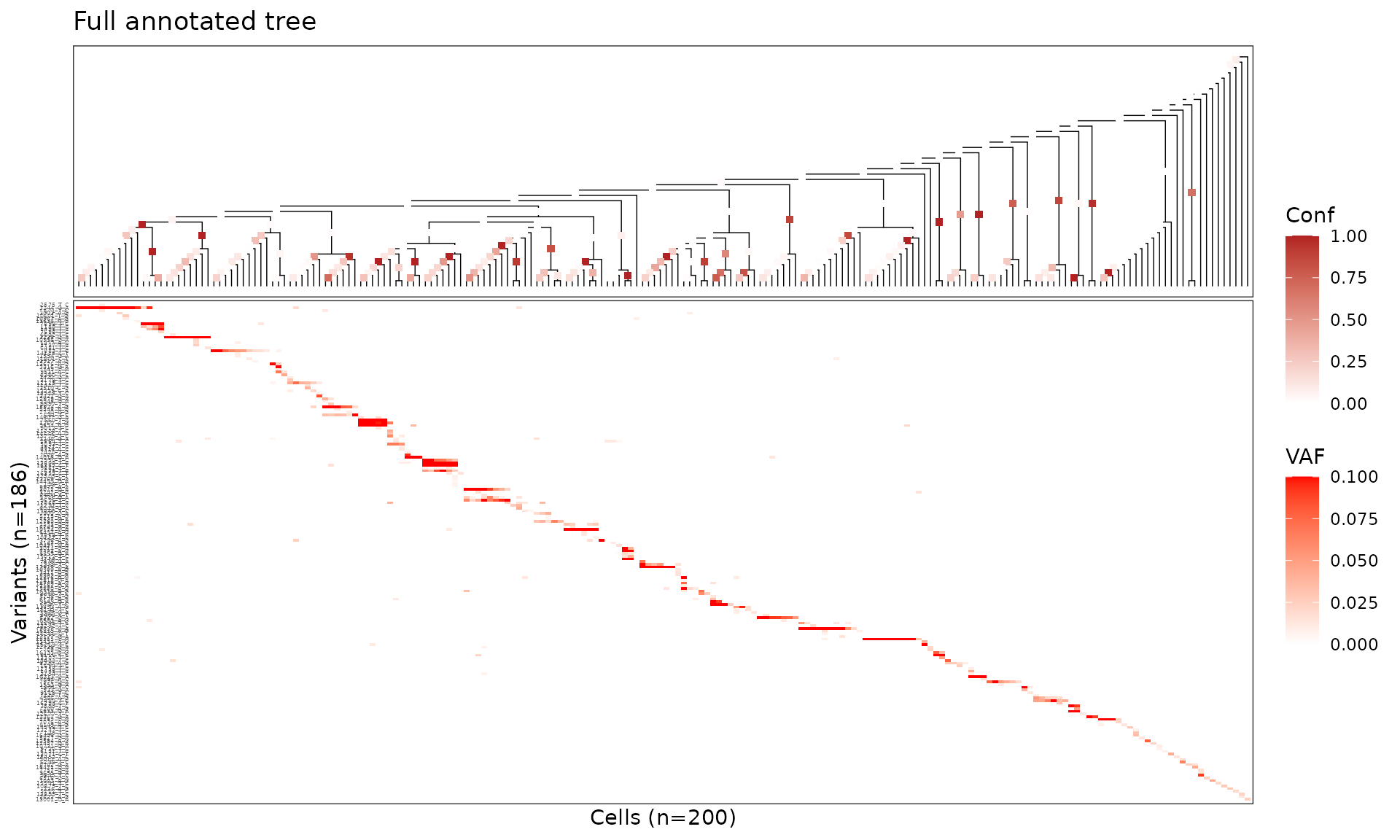
plot_phylo_heatmap2() displays the tree alongside a variant heteroplasmy heatmap. Setting node_conf = TRUE colours internal nodes by their confidence score.

plot_phylo_heatmap2(
  tree_annot,
  mut_dat,
  node_conf = TRUE,
  dot_size = 2,
  branch_length = FALSE,
  title = "Full annotated tree"
)

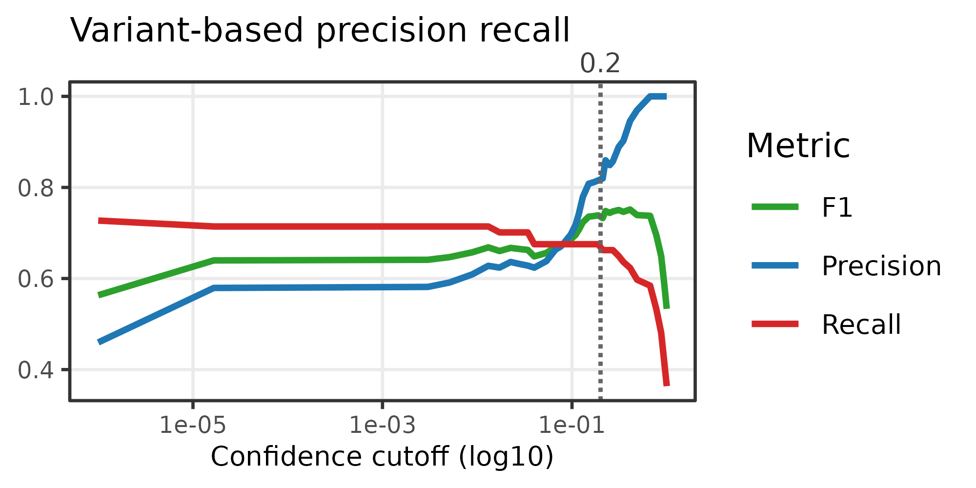
Diagnostic: variant precision–recall curve

compute_variant_pr_curve() compares variant-defined cell partitions against tree clades across a sweep of confidence cutoffs. This helps identify a threshold that balances precision (are the clades real?) and recall (are we keeping enough structure?).

pr_df <- compute_variant_pr_curve(tree_annot, mut_dat)
plot_prec_recall_vs_conf(
  pr_df,
  sample_name = "Variant-based precision recall",
  cutoff = 0.2
)

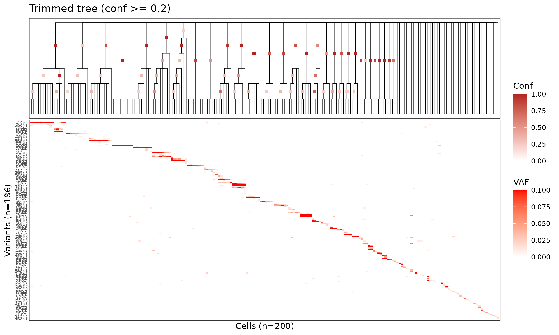
Trim tree

Collapse low-confidence nodes below the chosen threshold with trim_tree().

tree_trim <- trim_tree(tree_annot, conf = 0.2)

Visualize the trimmed tree — polytomies replace poorly supported splits.

plot_phylo_heatmap2(
  tree_trim,
  mut_dat,
  node_conf = TRUE,
  dot_size = 2,
  branch_length = FALSE,
  title = "Trimmed tree (conf >= 0.2)"
)

Clone assignment

assign_clones_polytomy() partitions tips into clones based on the polytomy structure of the trimmed tree.

clone_df <- assign_clones_polytomy(tree_trim)
head(clone_df)

## # A tibble: 6 × 6
##   cell               clade clade_node annot  size  frac
##   <chr>              <chr>      <int> <chr> <int> <dbl>
## 1 CAACTAATCATTGACA-1 1            202 1        15 0.075
## 2 GTTCATTTCGGTTTGG-1 1            202 1        15 0.075
## 3 ATGTAAGCAATTGCGC-1 1            202 1        15 0.075
## 4 GGGCAATAGGCCCAGT-1 1            202 1        15 0.075
## 5 CAGCCTAAGACAACAG-1 1            202 1        15 0.075
## 6 TAGGCTAGTCGAAGTC-1 1            202 1        15 0.075

Visualize clones

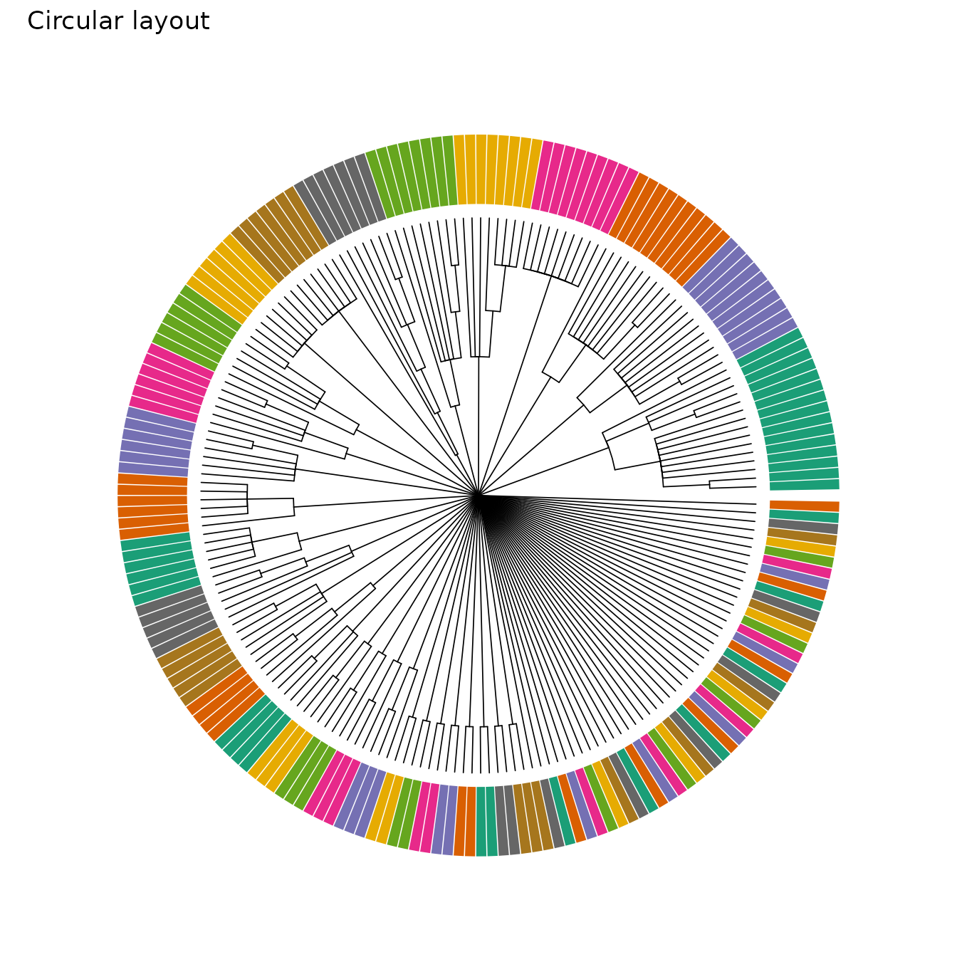
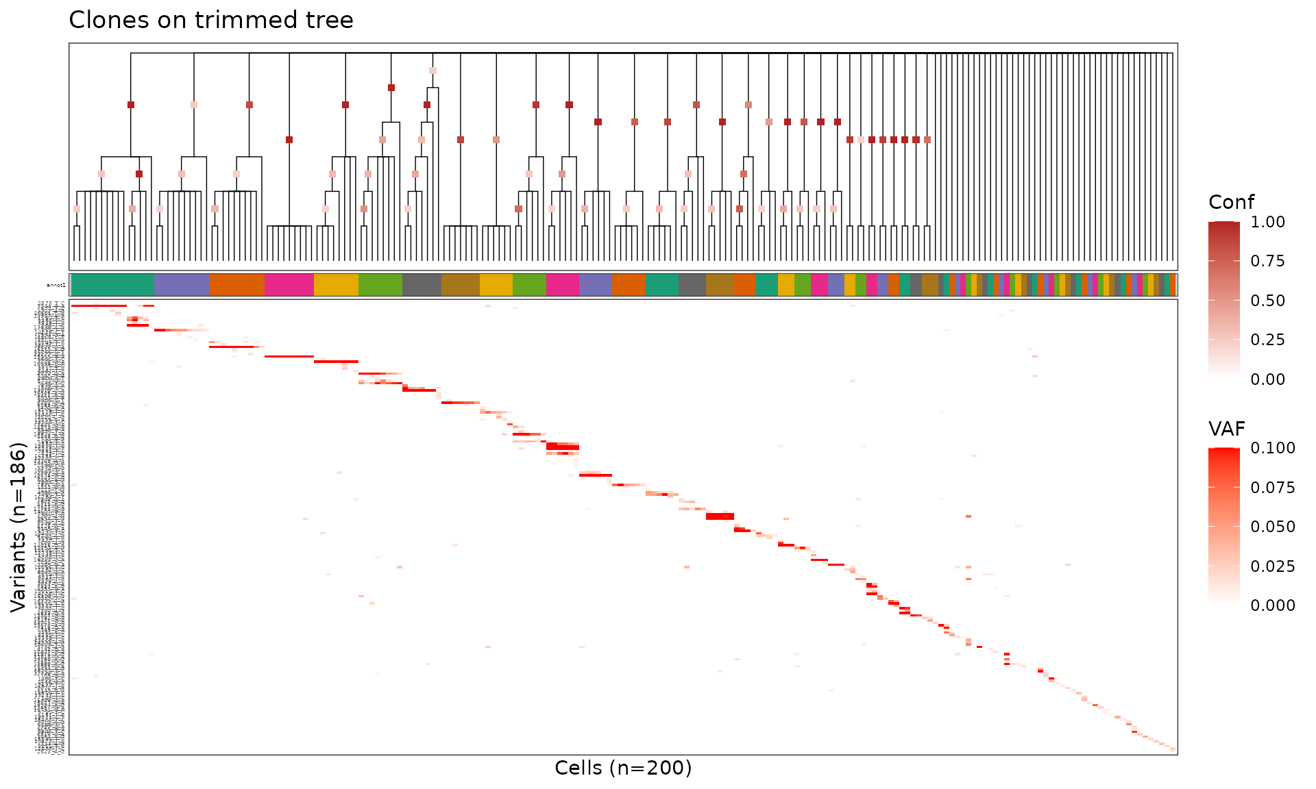
Colour cells by clone assignment on both a rectangular heatmap view and a circular layout.

clade_order <- unique(clone_df$clade)
clone_pal <- make_clade_pal(length(clade_order), labels = clade_order,
                            pal = "Dark2", cycle_len = 8, cycle_shift = 0)

plot_phylo_heatmap2(
  tree_trim,
  mut_dat,
  cell_annot = clone_df,
  annot_pal = clone_pal,
  node_conf = TRUE,
  dot_size = 2,
  branch_length = FALSE,
  title = "Clones on trimmed tree"
)

plot_phylo_circ(
  tree_trim,
  cell_annot = clone_df,
  annot_pal = clone_pal,
  annot_legend = FALSE,
  title = "Circular layout"
)