Overview
This vignette covers the main function and workflow of SCAVENGE. The standard processed input data including fine-mapped variants and single-cell epigenomic profiles. For fine-mapped variants of the trait of interest, we typically need information of genomic locations of variants and their corresponding posterior propability of causality. A peak-by-cell matrix of scATAC-seq profiles is needed. To walk through the workflow of SCAVENGE, we provided a blood cell trait of monocyte count and a 10X PBMC dataset as an example.
Load required packages
library(SCAVENGE)
library(chromVAR)
library(gchromVAR)
library(BuenColors)
library(SummarizedExperiment)
library(data.table)
library(dplyr)
library(BiocParallel)
library(BSgenome.Hsapiens.UCSC.hg19)
library(igraph)

set.seed(9527)
Load example data
The PBMC data was processed using ArchR package. The peak-by-cell count matrix and corresponding meta data were extracted and stored in a RangedSummarizedExperiment object (for more details please follow our paper). The typical input of fine-mapped data for SCAVENGE or g-chromVAR can be found here (https://github.com/sankaranlab/SCAVENGE-reproducibility/tree/main/data/finemappedtraits_hg19). You can use this (trait_import <- importBedScore(rowRanges(SE_pbmc5k), trait_file, colidx=5)) to import your fine-mapped data into SummarizedExperiment when you have your data ready (trait_file is the path of your file).
trait_import <- example_data(name="mono.PP001.bed")
SE_pbmc5k <- example_data(name="pbmc5k_SE.rda")
gchromVAR analysis
SE_pbmc5k <- addGCBias(object = SE_pbmc5k,
                       genome = BSgenome.Hsapiens.UCSC.hg19::BSgenome.Hsapiens.UCSC.hg19)
SE_pbmc5k_bg <- getBackgroundPeaks(object = SE_pbmc5k,
                                   niterations = 200)
SE_pbmc5k_DEV <- computeWeightedDeviations(object = SE_pbmc5k,
                                           weights = trait_import,
                                           background_peaks = SE_pbmc5k_bg)
Reformat results
z_score_mat <- data.frame(SummarizedExperiment::colData(SE_pbmc5k),
                          z_score=t(SummarizedExperiment::assays(SE_pbmc5k_DEV)[["z"]]) |> c())
head(z_score_mat)
## names x y color
## input1#GTCACGGAGCTCGGCT-1 input1#GTCACGGAGCTCGGCT-1 11.71388 1.903179 Mono-2
## input1#CTGAATGAGCAGAATT-1 input1#CTGAATGAGCAGAATT-1 -13.86186 -4.616170 T-1
## input1#CCTGCTACAATGGCAG-1 input1#CCTGCTACAATGGCAG-1 10.90323 1.913244 Mono-2
## input1#TCAGGTAAGAGCAGCT-1 input1#TCAGGTAAGAGCAGCT-1 -13.64482 -4.757390 T-1
## input1#GAGTGAGTCGGTCTCT-1 input1#GAGTGAGTCGGTCTCT-1 10.77266 1.872978 Mono-2
## input1#AGGCCCAAGTCTGCTA-1 input1#AGGCCCAAGTCTGCTA-1 -13.88653 -4.610587 T-1
## color2 sample cell_cluster z_score
## input1#GTCACGGAGCTCGGCT-1 C5 input1 C5 0.3950389
## input1#CTGAATGAGCAGAATT-1 C1 input1 C1 0.0984394
## input1#CCTGCTACAATGGCAG-1 C5 input1 C5 0.3504030
## input1#TCAGGTAAGAGCAGCT-1 C1 input1 C1 -2.7724179
## input1#GAGTGAGTCGGTCTCT-1 C5 input1 C5 -0.4360599
## input1#AGGCCCAAGTCTGCTA-1 C1 input1 C1 -2.1425049Generate the seed cell index (using the top 5% if too many cells are eligible)
seed_idx <- seedindex(z_score = z_score_mat$z_score,
                      percent_cut = 0.05)
## Cells with enriched P < 0.05: 612## Percent: 13.42%## The top 5% of cells (N=228) were selected as seed cellscalculate scale factor
scale_factor <- cal_scalefactor(z_score = z_score_mat$z_score,
                                percent_cut = 0.01)
## Scale factor is calculating from most enriched 1% of cells.Construct m-knn graph
Calculate tfidf-mat
peak_by_cell_mat <- SummarizedExperiment::assay(SE_pbmc5k)
tfidf_mat <- tfidf(bmat=peak_by_cell_mat,
                   mat_binary=TRUE,
                   TF=TRUE,
                   log_TF=TRUE)
## [info] binarize matrix## [info] calculate tf## [info] calculate idf## [info] fast log tf-idfCalculate lsi-mat
lsi_mat <- do_lsi(mat = tfidf_mat,
                  dims = 30)
## SVD analysis of TF-IDF matrixPlease be sure that there is no potential batch effects for
cell-to-cell graph construction. If the cells are from different samples
or different conditions etc., please consider using Harmony analysis
(HarmonyMatrix from Harmony
package). Typically you could take the lsi_mat as the input with
parameter do_pca = FALSE and provide meta data describing
extra data such as sample and batch for each cell. Finally, a
harmony-fixed LSI matrix can be used as input for the following
analysis.
Calculate m-knn graph
mutualknn30 <- getmutualknn(lsimat = lsi_mat,
                            num_k = 30)
Network propagation
np_score <- randomWalk_sparse(intM = mutualknn30,
                              queryCells = rownames(mutualknn30)[seed_idx],
                              gamma = 0.05)
Trait relevant score (TRS) with scaled and
normalized
A few cells are singletons are removed from further analysis, this will
lead very few cells be removed for the following analysis. You can
always recover those cells with a unified score of 0 and it will not
impact the following analysis.
omit_idx <- np_score==0
sum(omit_idx)
## [1] 23
mutualknn30 <- mutualknn30[!omit_idx, !omit_idx]
np_score <- np_score[!omit_idx]
TRS <- capOutlierQuantile(x = np_score,
                          q_ceiling = 0.95) |> max_min_scale()
TRS <- TRS * scale_factor
mono_mat <- data.frame(z_score_mat[!omit_idx, ],
                       seed_idx[!omit_idx],
                       np_score,
                       TRS)
head(mono_mat)
## names x y color
## input1#GTCACGGAGCTCGGCT-1 input1#GTCACGGAGCTCGGCT-1 11.71388 1.903179 Mono-2
## input1#CTGAATGAGCAGAATT-1 input1#CTGAATGAGCAGAATT-1 -13.86186 -4.616170 T-1
## input1#CCTGCTACAATGGCAG-1 input1#CCTGCTACAATGGCAG-1 10.90323 1.913244 Mono-2
## input1#TCAGGTAAGAGCAGCT-1 input1#TCAGGTAAGAGCAGCT-1 -13.64482 -4.757390 T-1
## input1#GAGTGAGTCGGTCTCT-1 input1#GAGTGAGTCGGTCTCT-1 10.77266 1.872978 Mono-2
## input1#AGGCCCAAGTCTGCTA-1 input1#AGGCCCAAGTCTGCTA-1 -13.88653 -4.610587 T-1
## color2 sample cell_cluster z_score
## input1#GTCACGGAGCTCGGCT-1 C5 input1 C5 0.3950389
## input1#CTGAATGAGCAGAATT-1 C1 input1 C1 0.0984394
## input1#CCTGCTACAATGGCAG-1 C5 input1 C5 0.3504030
## input1#TCAGGTAAGAGCAGCT-1 C1 input1 C1 -2.7724179
## input1#GAGTGAGTCGGTCTCT-1 C5 input1 C5 -0.4360599
## input1#AGGCCCAAGTCTGCTA-1 C1 input1 C1 -2.1425049
## seed_idx..omit_idx. np_score TRS
## input1#GTCACGGAGCTCGGCT-1 FALSE 3.804691e-05 0.213939514
## input1#CTGAATGAGCAGAATT-1 FALSE 2.209024e-07 0.001187911
## input1#CCTGCTACAATGGCAG-1 FALSE 6.088393e-05 0.342385858
## input1#TCAGGTAAGAGCAGCT-1 FALSE 2.220132e-07 0.001194159
## input1#GAGTGAGTCGGTCTCT-1 FALSE 4.785297e-05 0.269093513
## input1#AGGCCCAAGTCTGCTA-1 FALSE 2.572135e-07 0.001392142UMAP plots of cell type annotation and cell-to-cell graph
Cell type annotation
p <- ggplot(data=mono_mat, aes(x, y, color=color)) +
  geom_point(size=1, na.rm = TRUE) +
  pretty_plot() +
  theme(legend.title = element_blank()) +
  labs(x="UMAP 1",y="UMAP 2")
p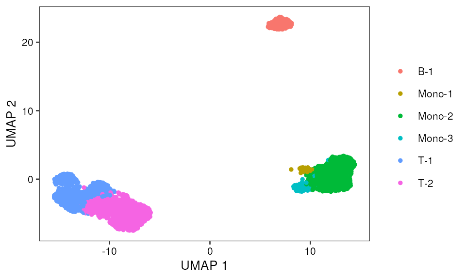
Visualize cell-to-cell graph if you have low-dimensional coordinates such as UMAP1 and UMAP2
mutualknn30_graph <- graph_from_adjacency_matrix(adjmatrix = mutualknn30,
                                                 mode = "undirected",
                                                 diag = FALSE)
igraph::plot.igraph(x = mutualknn30_graph,
                    vertex.size=0.8,
                    vertex.label=NA,
                    vertex.color=adjustcolor("#c7ce3d", alpha.f = 1),
                    vertex.frame.color=NA,
                    edge.color=adjustcolor("#443dce", alpha.f = 1),
                    edge.width=0.3, edge.curved=.5,
                    layout=as.matrix(data.frame(mono_mat$x, mono_mat$y)))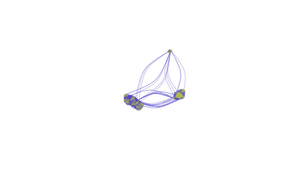
Comparsion before and after SCAVENGE analysis
- Z score based visualization
Scatter plot
p1 <- ggplot(data=mono_mat, aes(x, y, color=z_score)) +
geom_point(size=1, na.rm = TRUE, alpha = 0.6) +
scale_color_viridis_c() +
scale_alpha() +
pretty_plot() +
theme(legend.title = element_blank()) +
labs(x="UMAP 1", y="UMAP 2")
p1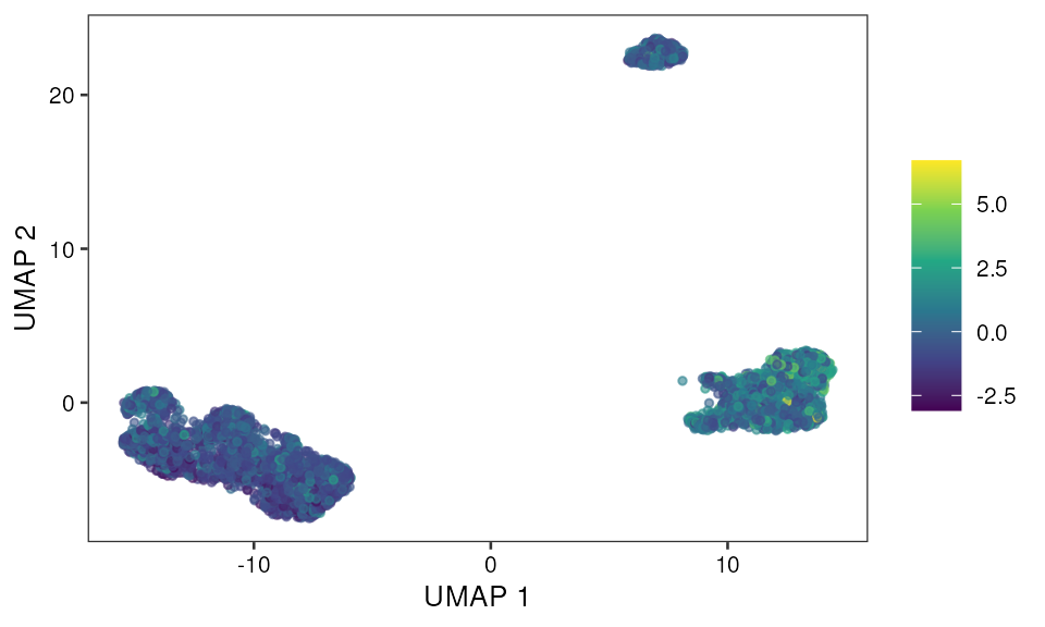 Bar plot
pp1 <- ggplot(data=mono_mat,  aes(x=color, y=z_score))  +
  geom_boxplot(aes(fill=color, color=color), outlier.shape=NA) +
  guides(fill=FALSE) +
  pretty_plot(fontsize = 10) +
  stat_summary(geom = "crossbar", width=0.65, fatten=0, color="black",
               fun.data = function(x){ return(c(y=median(x), ymin=median(x), ymax=median(x))) }) + theme(legend.position = "none")
pp1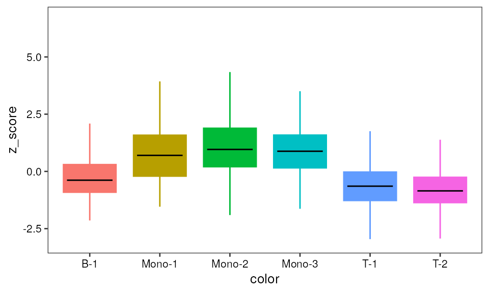
- SCAVENGE TRS based visualization
Scatter plot
p2 <- ggplot(data=mono_mat, aes(x, y, color=TRS)) +
geom_point(size=1, na.rm = TRUE, alpha = 0.6) +
scale_color_viridis_c() +
scale_alpha() + pretty_plot() +
theme(legend.title = element_blank()) +
labs(x="UMAP 1", y="UMAP 2")
p2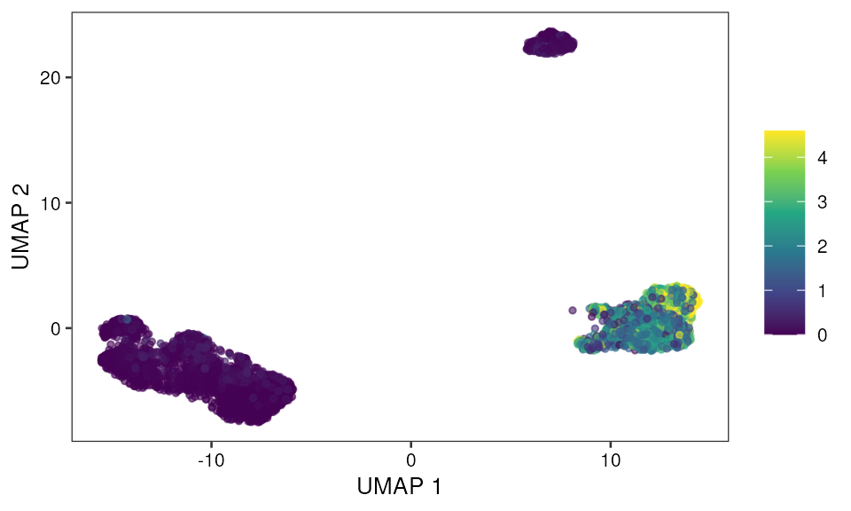 Bar plot
pp2 <- ggplot(data=mono_mat,  aes(x=color, y=TRS))  +
  geom_boxplot(aes(fill=color, color=color), outlier.shape=NA) +
  guides(fill=FALSE) +
  pretty_plot(fontsize = 10) +
  stat_summary(geom = "crossbar", width=0.65, fatten=0, color="black", fun.data = function(x){ return(c(y=median(x), ymin=median(x), ymax=median(x))) }) + theme(legend.position = "none")
pp2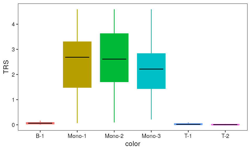
Trait relevant cell determination from permutation test
About 2 mins
please set @mycores >= 1 and @permutation_times >= 1,000 in the real
setting
mono_permu <- get_sigcell_simple(knn_sparse_mat=mutualknn30,
                                 seed_idx=mono_mat$seed_idx,
                                 topseed_npscore=mono_mat$np_score,
                                 permutation_times=100, # Increase to >=1000 in practice
                                 true_cell_significance=0.05,
                                 rda_output=FALSE,
                                 # mycores=8,# Increase in practice
                                 rw_gamma=0.05)
mono_mat2 <- data.frame(mono_mat, mono_permu)
Look at the distribution of statistically significant phenotypically enriched and depleted cells
Enriched cells
mono_mat2 |>
  dplyr::group_by(color) |>
  dplyr::summarise(enriched_cell=sum(true_cell_top_idx)) |>
  ggplot(aes(x=color, y=enriched_cell, fill=color)) +
  geom_bar(stat="identity") +
  theme_classic()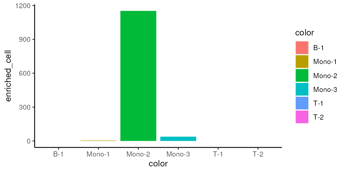
Depleted cells
mono_mat2$rev_true_cell_top_idx <- !mono_mat2$true_cell_top_idx
mono_mat2 |>
  dplyr::group_by(color) |>
  dplyr::summarise(depleted_cell=sum(rev_true_cell_top_idx)) |>
  ggplot(aes(x=color, y=depleted_cell, fill=color)) +
  geom_bar(stat="identity") +
  theme_classic()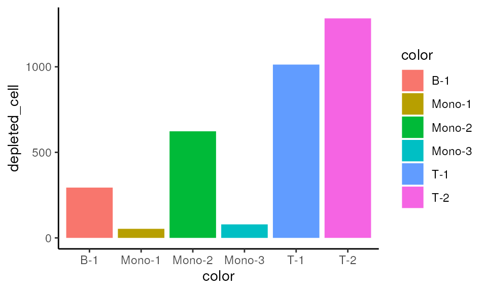
Sesssion info
utils::sessionInfo()## R Under development (unstable) (2023-02-16 r83857)
## Platform: x86_64-pc-linux-gnu (64-bit)
## Running under: Ubuntu 22.04.1 LTS
##
## Matrix products: default
## BLAS: /usr/lib/x86_64-linux-gnu/openblas-pthread/libblas.so.3
## LAPACK: /usr/lib/x86_64-linux-gnu/openblas-pthread/libopenblasp-r0.3.20.so; LAPACK version 3.10.0
##
## locale:
## [1] LC_CTYPE=en_US.UTF-8 LC_NUMERIC=C
## [3] LC_TIME=en_US.UTF-8 LC_COLLATE=en_US.UTF-8
## [5] LC_MONETARY=en_US.UTF-8 LC_MESSAGES=en_US.UTF-8
## [7] LC_PAPER=en_US.UTF-8 LC_NAME=C
## [9] LC_ADDRESS=C LC_TELEPHONE=C
## [11] LC_MEASUREMENT=en_US.UTF-8 LC_IDENTIFICATION=C
##
## time zone: UTC
## tzcode source: system (glibc)
##
## attached base packages:
## [1] stats4 stats graphics grDevices utils datasets methods
## [8] base
##
## other attached packages:
## [1] igraph_1.4.0 BSgenome.Hsapiens.UCSC.hg19_1.4.3
## [3] BSgenome_1.67.4 rtracklayer_1.59.1
## [5] Biostrings_2.67.0 XVector_0.39.0
## [7] BiocParallel_1.33.9 dplyr_1.1.0
## [9] data.table_1.14.8 SummarizedExperiment_1.29.1
## [11] Biobase_2.59.0 GenomicRanges_1.51.4
## [13] GenomeInfoDb_1.35.15 IRanges_2.33.0
## [15] S4Vectors_0.37.3 BiocGenerics_0.45.0
## [17] MatrixGenerics_1.11.0 matrixStats_0.63.0
## [19] BuenColors_0.5.6 ggplot2_3.4.1
## [21] MASS_7.3-58.2 gchromVAR_0.3.2
## [23] chromVAR_1.21.0 SCAVENGE_1.0.2
## [25] BiocStyle_2.27.1
##
## loaded via a namespace (and not attached):
## [1] jsonlite_1.8.4 magrittr_2.0.3
## [3] farver_2.1.1 rmarkdown_2.20
## [5] fs_1.6.1 BiocIO_1.9.2
## [7] zlibbioc_1.45.0 ragg_1.2.5
## [9] vctrs_0.5.2 memoise_2.0.1
## [11] Rsamtools_2.15.1 RCurl_1.98-1.10
## [13] htmltools_0.5.4 CNEr_1.35.0
## [15] sass_0.4.5 pracma_2.4.2
## [17] bslib_0.4.2 htmlwidgets_1.6.1
## [19] desc_1.4.2 plyr_1.8.8
## [21] plotly_4.10.1 cachem_1.0.6
## [23] GenomicAlignments_1.35.0 mime_0.12
## [25] lifecycle_1.0.3 pkgconfig_2.0.3
## [27] Matrix_1.5-3 R6_2.5.1
## [29] fastmap_1.1.0 GenomeInfoDbData_1.2.9
## [31] shiny_1.7.4 digest_0.6.31
## [33] colorspace_2.1-0 TFMPvalue_0.0.9
## [35] AnnotationDbi_1.61.0 rprojroot_2.0.3
## [37] irlba_2.3.5.1 textshaping_0.3.6
## [39] RSQLite_2.3.0 labeling_0.4.2
## [41] seqLogo_1.65.0 fansi_1.0.4
## [43] httr_1.4.4 compiler_4.3.0
## [45] withr_2.5.0 bit64_4.0.5
## [47] DBI_1.1.3 highr_0.10
## [49] R.utils_2.12.2 poweRlaw_0.70.6
## [51] DelayedArray_0.25.0 rjson_0.2.21
## [53] gtools_3.9.4 caTools_1.18.2
## [55] tools_4.3.0 httpuv_1.6.9
## [57] R.oo_1.25.0 glue_1.6.2
## [59] restfulr_0.0.15 promises_1.2.0.1
## [61] grid_4.3.0 reshape2_1.4.4
## [63] TFBSTools_1.37.0 generics_0.1.3
## [65] gtable_0.3.1 tzdb_0.3.0
## [67] R.methodsS3_1.8.2 nabor_0.5.0
## [69] tidyr_1.3.0 hms_1.1.2
## [71] utf8_1.2.3 RANN_2.6.1
## [73] pillar_1.8.1 stringr_1.5.0
## [75] later_1.3.0 lattice_0.20-45
## [77] bit_4.0.5 annotate_1.77.0
## [79] tidyselect_1.2.0 DirichletMultinomial_1.41.0
## [81] GO.db_3.16.0 miniUI_0.1.1.1
## [83] knitr_1.42 bookdown_0.32
## [85] xfun_0.37 DT_0.27
## [87] stringi_1.7.12 lazyeval_0.2.2
## [89] yaml_2.3.7 evaluate_0.20
## [91] codetools_0.2-19 tibble_3.1.8
## [93] BiocManager_1.30.19 cli_3.6.0
## [95] xtable_1.8-4 systemfonts_1.0.4
## [97] munsell_0.5.0 jquerylib_0.1.4
## [99] Rcpp_1.0.10 png_0.1-8
## [101] XML_3.99-0.13 parallel_4.3.0
## [103] ellipsis_0.3.2 pkgdown_2.0.7
## [105] readr_2.1.4 blob_1.2.3
## [107] bitops_1.0-7 viridisLite_0.4.1
## [109] scales_1.2.1 purrr_1.0.1
## [111] crayon_1.5.2 rlang_1.0.6
## [113] KEGGREST_1.39.0